The tool's static analysis is primarily used to initialize dynamic models. Figure 1 illustrates the complete initialization process through a sequence diagram.

The power system's initialization happens in two phases: first, the power system itself, and then the control systems of the units. The power system initialization is performed via a power-flow (PF) analysis, specifically using MATPOWER-FUBM. In this analysis, we only consider the grid structure, excluding any generation controllers. This is achieved by selecting the "Loadflow" block as the active choice within the grid variant system, which then treats dynamic models as commented blocks in Simulink.

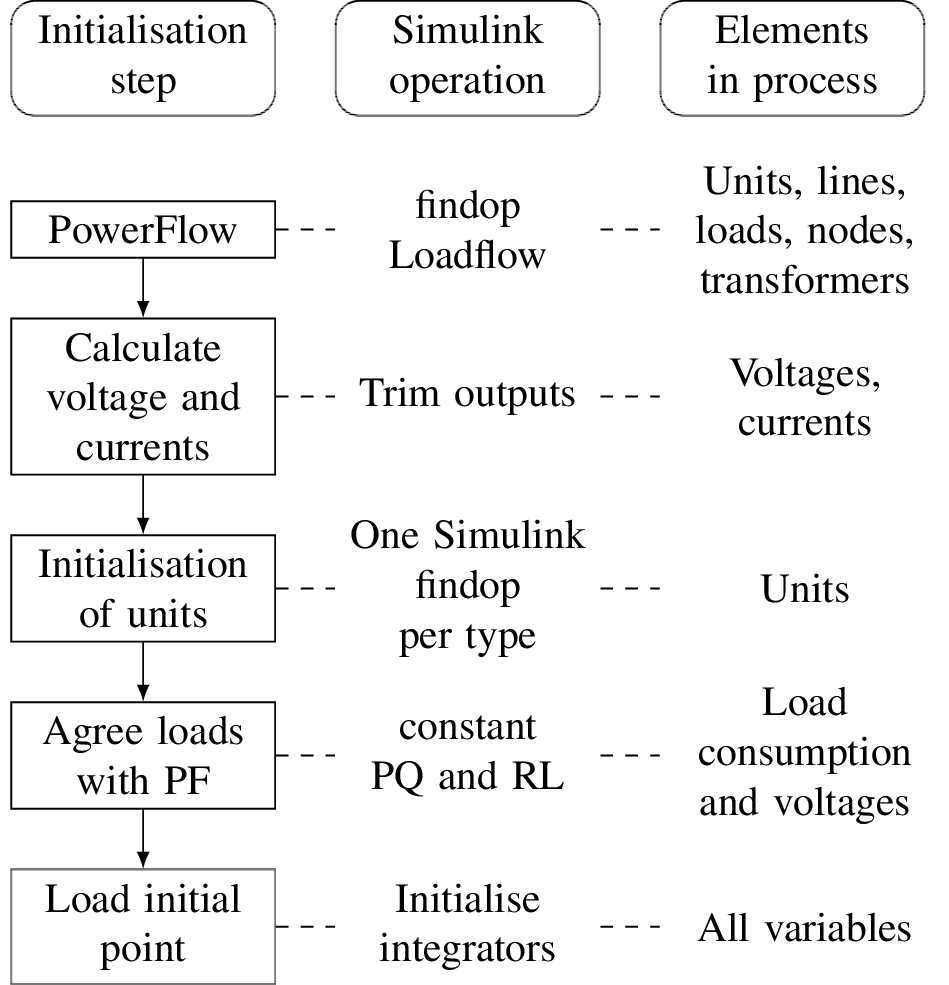
Loads are modeled as constant PQ loads, consuming the active and reactive power defined in the grid bus table. Buses are set as static parallel RC circuits, and lines as static series RL circuits. As before, users can select the complexity of the models for each element.

To solve the PF within the tool, we don't consider the voltage (magnitude and angle) of all buses in the grid table. Instead, the initial bus voltage is set to 1 pu in magnitude and 0 radians in angle. Generators can be configured as either PV or PQ. If set to PV, their voltage magnitude and injected active power are taken from their values in the grid table. If set to PQ, their injected active and reactive power are set to their values in the grid table. The first generator is designated as the slack generator, and its voltage magnitude is set to its value from the table.

To maintain consistency between static and dynamic models, the R and L values for loads are computed to consume the same active and reactive power as determined in the loadflow solution, based on the voltage at their connection point.